
Multivariable linear regression is all about taking in a set of data points (x0, x1, …,xn, y) and to be able to predict y values for some other data points (x0',x1',…,xn'). I'm giving an example here on how to do so in Python as well as computing the coefficient of determination (R2) to see how well the predictor variables model y.
All the following code is available with an MIT licence here.
Input#
Dataset#
The example data has been adapted from the Thunder Basin Antelope study found online here. The data contains four variables (each corresponding to a year), the first being the spring fawn count(/100), the second being annual precipitation (inches), the third being the winter severity index (1=mild, 5=severe), and the fourth variable (which is the one which will act as the dependent variable y) is the size of the adult antelope population(/100).
| Spring fawn count/100 | Annual precipitation(inches) | Winter severity index(1=mild;5=severe) | Size of adult antelope population/100 |
|---|---|---|---|
| 2.900000095 | 13.19999981 | 2 | 9.199999809 |
| 2.400000095 | 11.5 | 3 | 8.699999809 |
| 2 | 10.80000019 | 4 | 7.199999809 |
| 2.299999952 | 12.30000019 | 2 | 8.5 |
| 3.200000048 | 12.60000038 | 3 | 9.6 |
| 1.899999976 | 10.60000038 | 5 | 6.800000191 |
| 3.400000095 | 14.10000038 | 1 | 9.699999809 |
| 2.099999905 | 11.19999981 | 3 | 7.900000095 |
Goal#
The goal is to determine if the first three variables are good predictors of the adult antelope population size. And if they are, to make predictions of adult antelope population based on new data that only contains the first three variables (spring fawn count, annual precipitation and winter severity).
Output#
The below code handles the data acquisition from the csv files, and sends it to the MultivariableRegression class. There is the option to add a file to process a list of prediction data and whether to plot data.
import numpy as npimport csvimport mvr

class Main:
    filename  = "antelopestudy.csv"    predict   = "antelope_predict.csv"    delimiter = ','
    # Load CSV headers only    with open(filename) as file:        reader = csv.reader(file)        headers = next(reader)
    # Load remaining CSV data    data = np.loadtxt(filename, delimiter=delimiter, skiprows=1)    prediction_data = np.loadtxt(predict, delimiter=delimiter, skiprows=1)
# Perform the regression r = mvr.MultiVariableRegression(data, headers, estimates=prediction_data) r.plotData()Results#
An analysis of variance test is run on the data. The analysis is run with a null hypothesis to check whether the population regression coefficients (A0, A1, A2) are 0. From the output, A0 (spring fawn count) is found to be a good predictor of the dependent variable. However the null hypothesis is accepted for both A1 (annual precipitation) and A2 (winter severity index), meaning we cannot say with 95% confidence that annual precipitation and the winter severity affects the adult antelope population.
Note
With significance of 95%, there is a 5% chance we reject the null hypothesis when it is true.
Running Analysis of Variance with given significance:0.95Null hypothesis: A_0...A_n are all 0Null hypotehesis rejected 6.59 < 27.1At least one A_x is not 0 with certainty 0.95Null hypotehesis rejected 6.59 < 11.6A_0 is not 0 with certainty 0.95Null hpothesis accepted6.59 > 2.29A_1 is 0 with certainty 0.95Null hpothesis accepted6.59 > 5.4A_2 is 0 with certainty 0.95For predictor variables: (0,): regression = [1.77142829 3.97714348]R^2 = 0.8615637849525227For predictor variables: (1,): regression = [ 0.78979077 -1.05710652]R^2 = 0.7837637022913508For predictor variables: (2,): regression = [-0.72183902 10.52528711]R^2 = 0.6494867453327626For predictor variables: (0, 1): regression = [1.35202677 0.21051042 2.50211306]R^2 = 0.8457378818812388For predictor variables: (0, 2): regression = [ 1.33311064 -0.27133953 5.86399668]R^2 = 0.89672011835548For predictor variables: (1, 2): regression = [ 0.69234295 -0.10668834 0.42265053]R^2 = 0.7445482721426719For predictor variables: (0, 1, 2): regression = [ 2.19667031 -0.70400663 -0.60502981 13.11734799]R^2 = 0.917920937434756x_n [ 2.5 14. 3. ] y_hat 6.94 ci 2.67 pi 2.8 with confidence 0.95Graphs of the correlation#
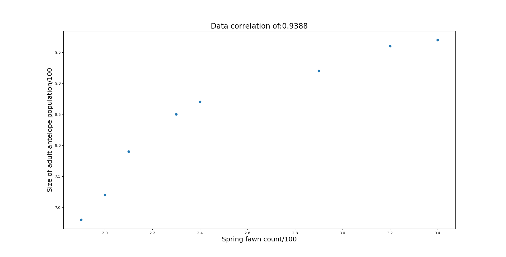
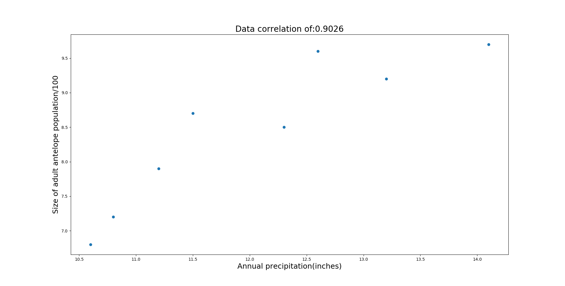
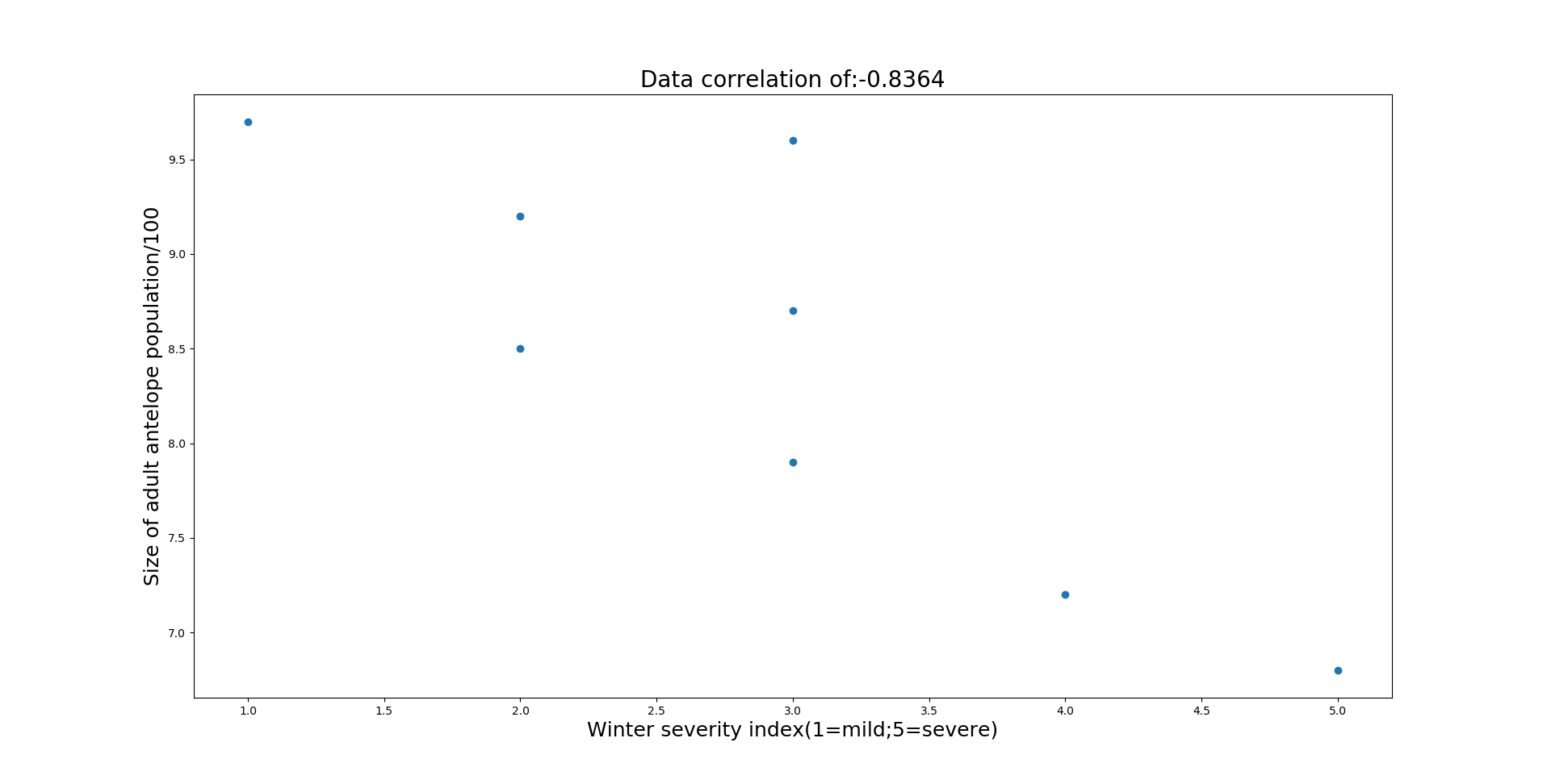
Additionally you can see the coefficient of determination (R2) is highest for the 0th predictor (spring fawn count). Based on this information, more data needs to be gathered to see if annual precipitation and winter severity can be a good indicator of population size.
Regression on spring fawn count#
The regression can be run again, using only the spring fawn count as the only independent variable. It is possible to quickly make a new dataset by making use of cut, to select columns 1 and 4. Then the main file gets updated to handle the new file, and the prediction file.
cat antelopestudy.csv | cut -d"," -f1,4 > antelopestudy_2.csv Output#
Running Analysis of Variance with given significance:0.95Null hypothesis: A_0...A_n are all 0Null hypotehesis rejected 5.99 < 44.6Atleast one A_x is not 0 with certainty 0.95For predictor variables: (0,): regression = [1.77142829 3.97714348]R^2 = 0.8615637849525227x_n [2.5] y_hat 8.41 ci 0.347 pi 1.04 with confidence 0.95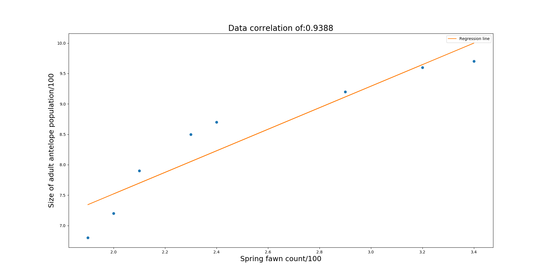
The output regression equation is 1.77a + 3.98. So for some given fawn count, an estimate can be given of the adult antelope count.
So given the fact that the spring fawn count is 250, an estimate is given of 841 adult antelopes. If there were many fawn counts of 250, the expected mean adult antelopes is expected to fall within the predicted (841) plus or minus the confidence interval (0.347) which represents a hundered. So with 0.95 confidence and spring fawn count of 250, the mean adult antelopes is expected to fall within 841+-35.
With observed readings (with 0.95 confidence) falling in 841+-104.
Source Code#
Again all the source code is available on GitHub under a MIT licence.
import numpy as npimport matplotlib.pyplot as pltimport itertools
import mvr_calc
class MultiVariableRegression:    """    Class to manage the multivariable regression, holding a data class,    which has it's own calculation class to handle regression calculations.    """
    class Data:        """Holds the raw numerical data for the regression calculations"""        def sanityCheck(self):            """            Test statistics rely on the degrees of freedom being            greater than 0, Having more data than the number of            variable predictors (x.. x_n) by atleast 2 will satisfy            the sanity check.            """            if self.df > 0:                self.sane = True
        def populateMetaData(self):            self.ndim  = self.c.getMatrixWidth(self.x)            self.ndata = self.y.size            self.df    = self.ndata - self.ndim - 1
            self.x_matrix = self.c.addOnesToData(self.x, self.ndata, self.ndim)
        def populateVariance(self):            self.y_bar = self.c.calcAverage(self.y)            self.x_bar = self.c.calcAverage(self.x)
            self.y_variance = self.c.calcVariance(self.y,self.y_bar)            self.x_variance = self.c.calcVariance(self.x,self.x_bar).reshape(                self.ndata, self.ndim)
            self.y_variance_sq = self.c.calcSumProduct(                self.y_variance,self.y_variance)
            self.x_variance_sq = np.zeros(self.ndim)            self.x_y_variance  = np.zeros(self.ndim)
            for n in range(0, self.ndim):                x_var = self.x_variance[:,n]                self.x_variance_sq[n] = self.c.calcSumProduct(                    x_var, x_var)                self.x_y_variance[n]  = self.c.calcSumProduct(                    x_var, self.y_variance)
        def populateCorrelation(self):            self.correlation = self.c.calcCorrelation(                self.ndim,                self.x_y_variance,                self.x_variance_sq,                self.y_variance_sq)
        def populateRegression(self):            self.s_matrix = self.c.findSMatrix(self.x_matrix)            self.regression = self.c.calcRegression(                self.s_matrix, self.x_matrix, self.y)
        def populateEstimationData(self):            self.y_hat   = np.dot(self.x_matrix, self.regression)            self.y_error = self.y - self.y_hat
            self.sum_errors_sq = self.c.calcSumProduct(                self.y_error, self.y_error)
            self.adjusted_R_sq = self.c.findAdjustedRSquared(                self.sum_errors_sq, self.y_variance_sq, self.ndata, self.df)
        def __init__(self,x,y,c):            self.x = x            self.y = y            self.c = c            self.populateMetaData()            self.sanityCheck()            if self.sane:                self.populateVariance()                self.populateCorrelation()                self.populateRegression()                self.populateEstimationData()
    def ANOVA(self,core_data,significance):        """        Run the analysis of variance test on the data. The analysis        is run with a null hypothesis to check whether the population        regression coefficients (A_0 ... A_n) are 0. Such that the data        follows a normal distribution with mean B and standard deviation        sigma. By rejecting the hypothesis, we can say with the given        significance the x dimensions do affect the y data. And        uses the F distribution to determine the critical value.
        Run once for All A_0,... A_n being 0, which can be rejected        if any A is not 0. Then run for each A_x.        """        print(f'Running Analysis of Variance with given significance:'              + f'{significance}\nNull hypothesis: A_0...A_n are all 0')
        test_statistic = self.c.calcTestStatisticAllX(            core_data.y_variance_sq,            core_data.sum_errors_sq,            core_data.ndim,            core_data.df)
        critical_value = core_data.c.findCriticalFValue(            core_data.ndim,            core_data.df,            significance)
        if critical_value < test_statistic:            print(f'Null hypotehesis rejected '                  + f'{critical_value:.3} < {test_statistic:.3}\n'                  + f'Atleast one A_x is not 0 with certainty {significance}')        else:            print(f'Null hpothesis accepted'                  + f'{critical_value:.3} > {test_statistic:.3}\n'                  + f'All A_x are 0 with certainty {significance}')
        if core_data.ndim > 1:            for n in range(0,core_data.ndim):                test_statistic = self.c.calcTestStatisticSingleX(                    core_data.regression,                    core_data.s_matrix,                    core_data.sum_errors_sq,                    n,                    core_data.df)
                critical_value = core_data.c.findCriticalFValue(                    core_data.ndim,                    core_data.df,                    significance)
                if critical_value < test_statistic:                    print(f'Null hypotehesis rejected '                          + f'{critical_value:.3} < {test_statistic:.3}\n'                          + f'A_{n} is not 0 with certainty {significance}')                else:                    print(f'Null hpothesis accepted'                          + f'{critical_value:.3} > {test_statistic:.3}\n'                          + f'A_{n} is 0 with certainty {significance}')

    def roundRobin(self):        """        Calculate the adjusted R^2 value for all combinations of        predictor variables, to determine which predictor variables        are best suited to the regression.        """        # Starting with 1 predictor variable up to n variables        for n in range(0, self.core_data.ndim):            # Generate all combinations of predictor variables            for i in itertools.combinations(range(0, self.core_data.ndim), n+1):                x = self.core_data.x[:,i]                sub_data = self.Data(x, self.core_data.y, self.c)
                print(f'For predictor variables: {i}'                      + f': regression = {sub_data.regression}'                      + f'R^2 = {sub_data.adjusted_R_sq}')

    def plotData(self):        """        Plot each predictor variable against y, showing the correlation        co-efficient for each variable. Additionally plots the regression        line if there is only one predictor variable.
        """        for n in range(0,self.core_data.ndim):            #plt.subplot(self.core_data.ndim, 1, n+1)            plt.figure(n)            x = self.core_data.x[:,n]            y = self.core_data.y            plt.plot(x,y,'o')
            plt.title(f'Data correlation of:'                      + f'{self.core_data.correlation[n]:.4}',                      fontsize=20)            plt.ylabel(f'{self.headers[-1]}',fontsize=18)            plt.xlabel(f'{self.headers[n]}',fontsize=18)

        # Regression line only makes sense to plot with 1 predictor variable        if self.core_data.ndim == 1:            a = self.core_data.regression[[n,self.core_data.ndim]]            x_matrix= self.c.addOnesToData(x, x.size, 1)            y_hat = np.dot(x_matrix, a)            plt.plot(x, y_hat, '-',label='Regression line')            plt.legend()
        plt.show()
    def estimateData(self):        """        For a given input list of data, provide an estimate y value,        along with a        confidence interval: (the interval of the mean y value),        prediction_interval: (the interval of predicted values).        """        if self.estimates is not None:            n = self.estimates.size // self.core_data.ndim            x = self.c.addOnesToData(self.estimates, n, self.core_data.ndim)
            y_hat = np.dot(x, self.core_data.regression)
            fval = self.c.findCriticalFValue(                1, self.core_data.df, self.confidence)
            for i in range(0,n):                x_n = x[i,:-1]
                mahalanobis_distance = self.c.getMahalanobisDistance(x_n,                    self.core_data.x_bar,                    self.core_data.ndim,                    self.core_data.ndata,                    self.core_data.s_matrix)
                # fval, sum_errors_sq, df, ndata, mahalanobis_distance):                confidence_interval = self.c.getConfidenceInterval(                    self.core_data.sum_errors_sq,                    self.core_data.df,                    self.core_data.ndata,                    mahalanobis_distance,                    fval)
                prediction_interval = self.c.getPredictionInterval(                    self.core_data.sum_errors_sq,                    self.core_data.df,                    self.core_data.ndata,                    mahalanobis_distance,                    fval)
                # TODO: add table formatting before loop                print(f'x_n {x_n} y_hat {y_hat[i]:.3}'                      + f' ci {confidence_interval[0,0]:.3}'                      + f' pi {prediction_interval[0,0]:.3}'                      + f' with confidence {self.confidence:.3}')

    def populateData(self):        if not self.data_populated:            self.core_data = self.Data(self.data[:,0:-1],self.data[:,-1],self.c)            data_populated = True
    def runAnalysisOfVariance(self, significance):         self.ANOVA(self.core_data,significance)
    def __init__(self, data, headers, confidence=0.95, estimates=None):        self.data_populated = False        self.data = data        self.confidence = confidence        self.c = mvr_calc.MVRCalculator()        self.headers = headers        self.estimates = estimates
        self.populateData()
self.runAnalysisOfVariance(self.confidence) self.roundRobin() self.estimateData()import numpy as npfrom scipy.stats import f
class MVRCalculator: """ Class holds the calculations needed to perform the regression on some data. Used to seperate out the data and calculations. """ @staticmethod def searchValue(f, target, tolerance=0.000001, start=0, step_size=1, damping=0.5): """ Finds x for a given target y, for a given linear function f(x). Works iteratively through values of x to find the target f(x) value, once the target is 'found', the step gets reversed and damped until the target is found within the given tolerance. """ def stepDirection(increasing, lower): """ Finds whether x should increase of decrease, depending if the f(x) function is an increasing or decreasing function and if f(x_0) is lower than f(x_target) """ if (increasing and lower) or (not increasing and not lower): return 1 else: return -1
x,error,a0,a1 = start, tolerance+1, f(start), f(start+step_size) increasing, start_lower = a1 > a0, a0 < target
step_direction = stepDirection(increasing, start_lower) step = step_direction * step_size
while abs(error) > tolerance : x = x + step a = f(x)
error = target - a lower = error > 0
new_step_direction = stepDirection(increasing, lower)
# If true, the target x is between f(x) and f(x-step) if step_direction != new_step_direction: step_size = damping * step_size
step = new_step_direction * step_size return x
@staticmethod def addOnesToData(x,ndata,ndim): """Adds a column of 1s to a given input vector or matrix""" #if len(x.shape) == 1: # x = np.expand_dims(x, axis=0) x = x.reshape(ndata,ndim) return np.append(x,np.ones((ndata,1)), axis=1)
@staticmethod def calcSumProduct(vector1,vector2): """Returns the sum of the product of two vectors""" return np.sum(vector1 * vector2)
@staticmethod def calcCorrelation(ndim, x_y_variance, x_variance_sq, y_variance_sq): """ Calculates the correlation between x and y data for each x dimension """ coefficients = np.zeros(ndim) for n in range(0,ndim): coefficients[n] = x_y_variance[n] / np.sqrt( x_variance_sq[n] * y_variance_sq) return coefficients
@staticmethod def calcRegression(s_matrix,x_matrix,y): """Calculates the regression equation (a_0 -> a_n + b)""" return np.dot(s_matrix, np.dot(x_matrix.T, y))
@staticmethod def findSMatrix(x_matrix): return np.linalg.inv(np.dot(x_matrix.T,x_matrix))
@staticmethod def findAdjustedRSquared(sum_errors_sq,y_variance_sq,ndata,df): """ Finds R^2, adjusted for the fact that normally R^2 will increase for added predictor variables regardless if the variable is a good predictor or not. """ return 1 - ((sum_errors_sq / df) / (y_variance_sq / (ndata - 1)))
@staticmethod def getMahalanobisDistance(x_n, x_bar, ndim, ndata, s_matrix): """Get the mahalanobis distance of a given x_n""" x = (x_n - x_bar).reshape(ndim,1) return np.dot(x.T,np.dot(s_matrix[:-1,:-1],x)) * (ndata - 1)
@staticmethod def findCriticalFValue(ndim, df, significance): """ Find F distribution values, used as critical values in Analysis of variance tests. """ return MVRCalculator.searchValue(lambda z: f.cdf(z,ndim,df), significance)
@staticmethod def getConfidenceInterval( sum_errors_sq, df, ndata, mahalanobis_distance, fval): """ Interval range for the mean value of a predicted y, to account for the variance in the population data. With the confidence (e.g. 0.95) determined by fval. """ return np.sqrt(fval * (1/ndata + mahalanobis_distance / (ndata -1)) * (sum_errors_sq / df))
@staticmethod def getPredictionInterval( sum_errors_sq, df, ndata, mahalanobis_distance, fval): """ Interval range to give a probable range of future values. This range will be higher than the confidence interval, to account for the fact that the mean predicted value can vary by the confidence value, and then additionally the value can vary from that mean. """ return np.sqrt(fval * (1 + 1/ndata + mahalanobis_distance / (ndata - 1)) * (sum_errors_sq / df))
@staticmethod def getMatrixWidth(v): """Function to find the width of a given numpy vector or matrix""" if len(np.shape(v)) > 1: return np.shape(v)[1] else: return 1
@staticmethod def autoCorrelationTest(y_error, sum_errors,sq): """ Check for auto correlation in our y data using the Durbin-Watson statistic, a result lower than 1 may indicate the presence of autocorrelation. """ residual = y_error[1:] - y_error[:-1] return (MVRCalculator.calcSumProduct(residual, residual) / sum_errors_sq)
@staticmethod def calcAverage(m): return np.mean(m,axis=0)
@staticmethod def calcVariance(v,v_bar): return v - v_bar @staticmethod def calcTestStatisticAllX(y_variance_sq,sum_errors_sq,ndim,df): """ Calculate the test statistic for the analysis of variance where the Null hypothesis is that the population A_1 -> A_n are all equal to 0. Such that the null hypothesis gets rejected if any A_x != 0. """ return (((y_variance_sq - sum_errors_sq) / ndim) / (sum_errors_sq / df))
@staticmethod def calcTestStatisticSingleX(regression, s_matrix, sum_errors_sq, n, df): """ Calculate the test statistic for the analysis of variance where the Null hypothesis is that the population A_n is 0. Such that the null hypothesis gets rejected if A_n != 0. """ return (regression[n]**2 / s_matrix[n,n]) / (sum_errors_sq / df)